

source: upload.wikimedia.org/wikipedia/commons/3/31..
When implementing a neural network, backpropagation is arguably where it is more prone to mistakes. So, how cool would it be if we could implement something which would allow us to debug our neural nets easily. Here, we will see the method of Gradient Checking. Briefly, this methods consists in approximating the gradient using a numerical approach. If it is close to the calculated gradients, then backpropagation was implemented correctly. But there is a lot more to this, let us see that. Sometimes, it can been seen that the network get stuck over a few epochs and then continues to converge quickly. We will also see how we can solve this problem. Let us get started!
All the visualizations and latex code used in the blog is available here- Rishit-dagli/Debugging-Neural-Nets Learn how to debug your neural nets with gradient checking This repository contains the visualization and tex files for…github.com
Numerical approximation of Gradients
In order for us to build up to Gradient Checking we first need to see how we can numerically approximate gradients. I find it easy to explain with an example so let us take one function f(θ) = θ³. Let us see a graph of this function-

As you might have guessed a simple graph. Let us as usual start off with some value of θ for now we say θ = 1. So, now what we will do is nudge our θ not just to the right to get (θ + ϵ) but also nudge it to the left and get (θ-ϵ). For purpose example we will just say ϵ = 0.01 Let us now visualize this, ignore the scale in this graph, its just for demonstration purposes.

So now our point which said (θ-ϵ) is named B and the (θ + ϵ) is called C. And in this figure what we earlier used to do was use the triangle DEF, and computed the height over width for it which in this case is EF/DE . It turns out that you can get a much better estimate for the gradient if you use a bigger triangle from (θ + ϵ) and (θ-ϵ), to show you what I mean I refer to the triangle here in red-

So, there are some papers on Why using this bigger triangle gives us a better approximation of the gradient at θ, but for the scope of this article I would not go into them in great detail. Simply explaining, you now have two smaller triangles which you are taking into account here by using the bigger triangle-

So, we just saw why you should use the bigger triangle instead, having that done let us get to the maths for that triangle. If we see here we can simply say that
H = f(θ-ϵ) and,
F = f(θ+ϵ)
With these two results you can say that the height(h) of the bigger triangle is
h = f(θ+ϵ)-f(θ-ϵ)
With similar arguments you can also easily calculate that the width(w) of this triangle is-
w = 2 ⋅ ϵ
Two-sided derivatives
So, if you know a bit of derivatives you can easily infer-

Where g(θ) refers to the gradient.
Now let us check how true the equation we wrote above is by plugging in the values for the example we just discussed. So, I would get something like this.

Let us now calculate the actual derivative of this. As i know f(θ) = θ³, by simple derivatives g(θ)=3 ⋅ θ² and we get g(θ) = 3. We did a pretty good approximation with our approximation error just being 0.0001. Now let us see what we would get if we used the one sided traditional approach. If you would calculate it by the one sided difference you would end up with 3.0301 with an approximation error of 0.0301. So, we did a fantastic job here reducing our approximation error significantly!
You just saw that two-sided derivatives performed a lot better than the traditional approach. And so this gives you a much greater confidence that g of theta is probably a correct implementation of the derivative of f(θ). This sounds too good to be true! And there is a downside of this approach too. It turns out to run twice as slow as you were to use a one-sided approach. But I believe that in practice it is worth it to use this method because it is just much more accurate.
Going a bit deeper
Let us take a look back at the formal definition of derivatives.

Here an important thing to note is the limits. So, for non zero values of ϵ you could show that the error of this approximation is in the order of ϵ². And ϵ is a very small number which tends to 0. So, to sum up
error = O(ϵ²)
Here O refers to the order of.
But you could prove by simple mathematics that if you use the one sided derivative your error would be in order of ϵ or
error = O(ϵ)
Again ϵ is a very small number of course less than 1, so ϵ >> ϵ². So now you probably understand why you should use a double sided difference rather than a single sided difference and we will see how this helps us in gradient checking.
Gradient Checking
Gradient Checking is a pretty useful technique and has helped me easily debug or find bugs in my neural nets many times. And now we will see how you could use this wonderful technique to debug or verify that your implementation and the back propagation is correct. Not something new but let us quickly see a diagram of a single neuron as a refresher-

Remember that [x₁, x₂ ... x_n] go as input and for each of these we have parameters (w¹, b¹) (w², b²) … (wⁿ, bⁿ). So to implement gradient checking, the first thing you should do is take all your parameters and reshape them into a giant vector data. So, what you do is take all of these w’s and b’s and reshape them individually to be a vector. And then you concatenate all of these vectors into one giant vector called θ. SO now we can write our cost function J in the terms of θ like this-

So now our J or cost function would just be a function of θ.
Now with your w’s and b’s ordered the same way you could also take dw¹ , db¹ … dwⁿ , dbⁿ and concatenate them into a single big vector which we will call dθ of the same dimension as θ. We will do so with similar procedure that is we shape all dw’s into vectors as they are matrices and b ‘s are already vectors so then just concatenate them. Just a point which I feel could be helpful is that dimensions of w¹ are same as those of dw¹ and those b¹ are same as that of db¹ and so on. This also means you can use the same sort of resize and concatenation operation. So, now you might have a question, “Is dθ the gradient or slope of θ here?” We will discuss that in a few moments.
Implementing Grad Check
Remember we wrote J as a function of θ let us now write it something like this-

Having done this, let us go through a process for any some θ maybe θ₅. So what we would now do is calculate the approximate derivative for θ₅ precisely a partial derivative to the function J. Also note we would be using the earlier discussed two sided derivative for this. To represent this mathematically-

Now by the discussion about double sided derivatives earlier we can also say that this is approximately the partial derivative of J to θ₅ or-

Having this clear to us we can now repeat the same process not just for θ₅ but for all i such that i ∈ (1, n) . So a pseudo Python code for this would look like this-

Approaching an outcome
So, now we have two vectors dθ[approx] and dθ . ANd these should almost be equal to each other. But now we would have another problem which is “How can I figure out if two vectors are approximately equal?”
What I would do now is compute the Euclidean distance between two vectors. What we would do is take the sum of squares of elements of the differences and then compute a square root of this to get the Euclidean distance. The above sentence may seem confusing, and believe me, it is! Read it twice or thrice and move forward once you are very clear with that. We will further apply another method on this, we will normalize the lengths of these vectors. To do this we would simply add their individual lengths and divide the Euclidean distance of the difference with this. If you feel this confusing now, hang on an equation will just help you.

Note: Here I have used the conventional symbol for L₂ norm of the vector. If you are wondering why we normalized this distance, it was just in case one of these vectors was really large or really small.
Implementing Gradient Check in practice
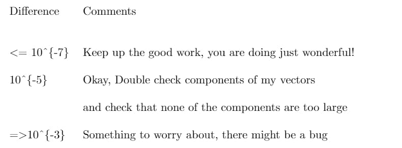
While implementing Gradient Check across a lot of projects I have observed that value of ϵ = 10⁻⁶ or 10⁻⁷ does the work most of the time. So, with the above mentioned similarity formula and this value of ϵ you find that formula yields a value smaller than 10⁻⁷ or 10⁻⁸, that is wonderful. It means your derivative approximation is very likely correct. If it is 10⁻⁵ I would say it is okay. But I would double check components of my vectors and check that none of the components are too large and if some of the components of this difference are very large maybe you have a bug. If it gives you 10⁻³ then I would be very much concerned and maybe there is a bug somewhere. In case you get bigger values than this something is really wrong! And you should probably look at the individual components of θ. Doing so you might find a value of dθ[i] which is very different from dθ[approx.] and use that to track down to find which of your derivative is incorrect.
I made a wonderful table for you to refer while making your ML applications-
 Reference table
In an ideal scenario what you would do when implementing a neural network, what often happens is you will implement forward propagation, implement backward propagation. And then you might find that this grad check has a relatively big value. And then suspect that there must be a bug, go in, debug, . And after debugging for a while, If you find that it passes grad check with a small value, then you can be much more confident that it’s then correct (and also get a sense of relief :) ). This particular method has often helped me find bugs in my neural network too and I would advise you to use this while debugging your nets too.
Some more Tips
- Do not use in training, only to debug
The grad check in each epoch will make it very slow
- If algorithm fails gradient check look at the components
Looking at the components would help a lot if your algorithm fails grad check. Sometimes it may also give you hints on where the bug might be.
- Regularization
If your J or cost function has an additional regularization term, then you would also calculate your derivatives for that and add them
- A different strategy for dropouts
What dropouts do is they randomly remove some neurons which make it hard to get a cost function on which they perform gradient descent. t turns out that dropout can be viewed as optimizing some cost function J, but it’s cost function J defined by summing over all exponentially large subsets of nodes they could eliminate in any iteration. So the cost function J is very difficult to compute, and you’re just sampling the cost function every time you eliminate different random subsets in those we use dropout. So it’s difficult to use grad check to double check your computation with dropouts. So what I usually do is implement grad check without dropout. So if you want, you can set keep-prob and dropout to be equal to 1.0. And then turn on dropout and hope that my implementation of dropout was correct.
You could also do this with some pretty elegant Taylor expansions but we will not go into that here.
Concluding
And that was it, you just saw how you could easily debug your neural networks and find problems in them very easily. I hope gradient checking will help you find problems or debug you nets just like it helped me
About Me
Hi everyone I am Rishit Dagli
LinkedIn — linkedin.com/in/rishit-dagli-440113165/
Website — rishit.tech
If you want to ask me some questions, report any mistake, suggest improvements, give feedback you are free to do so by mailing me at —
hello@rishit.tech