Extending what Convolutional nets can do

All the code used here is available in my GitHub repository here.

This is the fourth part of the series where I post about TensorFlow for Deep Learning and Machine Learning. In the earlier blog post, you saw a Convolutional Neural Network for Computer Vision. It did the job pretty nicely. This time you’re going to improve your skills with some real-life data sets and apply the discussed algorithms on them too. I believe in hands-on coding so we will have many exercises and demos which you can try yourself too. I would recommend you to play around with these exercises and change the hyper-parameters and experiment with the code. If you have not read the previous article consider reading it once before you read this one here. This one is more like a continuation of that.

Hands on with CNN

You can find the notebook used by me here. Again, you can download the notebook if you are using a local environment and if you are using Colab, you can click on opeen in colab button.

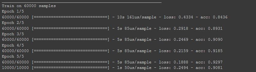
This is a really nice way to improve our image recognition performance. Let’s now look at it in action using a notebook. Here’s the same neural network that you used before for loading the set of images of clothing and then classifying them. By the end of epoch five, you can see the loss is around 0.34, meaning, your accuracy is pretty good on the training data.

Output with DNN

It took just a few seconds to train, so that’s not bad. With the test data as before and as expected, the losses a little higher and thus, the accuracy is a little lower.

So now, you can see the code that adds convolutions and pooling. We’re going to do 2 convolutional layers each with 64 convolutions, and each followed by a max pooling layer.

You can see that we defined our convolutions to be three-by-three and our pools to be two-by-two. Let’s train. The first thing you’ll notice is that the training is much slower. For every image, 64 convolutions are being tried, and then the image is compressed and then another 64 convolutions, and then it’s compressed again, and then it’s passed through the DNN, and that’s for 60,000 images that this is happening on each epoch. So it might take a few minutes instead of a few seconds. To remedy this what you can do is use a GPU. How to do that in Colab?

All you need to do is Runtime > Change Runtime Type > GPU. A single layer would now take approximately 5–6 seconds.

Output with the Convolutions and max poolings

Now that it’s done, you can see that the loss has improved a little it’s 0.25 now. In this case, it’s brought our accuracy up a bit for both our test data and with our training data. That’s pretty cool, right?

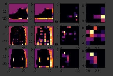
Now, this is a really fun visualization of the journey of an image through the convolutions. First, I’ll print out the first 100 test labels. The number 9 as we saw earlier is a shoe or boots. I picked out a few instances of this whether the zero, the 23rd and the 28th labels are all nine. So let’s take a look at their journey.

The visualization

The Keras API gives us each convolution and each pooling and each dense, etc. as a layer. So with the layers API, I can take a look at each layer’s outputs, so I’ll create a list of each layer’s output. I can then treat each item in the layer as an individual activation model if I want to see the results of just that layer. Now, by looping through the layers, I can display the journey of the image through the first convolution and then the first pooling and then the second convolution and then the second pooling. Note how the size of the image is changing by looking at the axes. If I set the convolution number to one, we can see that it almost immediately detects the laces area as a common feature between the shoes.

So, for example, if I change the third image to be one, which looks like a handbag, you’ll see that it also has a bright line near the bottom that could look like the soul of the shoes, but by the time it gets through the convolutions, that’s lost, and that area for the laces doesn’t even show up at all. So this convolution definitely helps me separate issue from a handbag. Again, if I said it’s a two, it appears to be trousers, but the feature that detected something that the shoes had in common fails again. Also, if I changed my third image back to that for shoe, but I tried a different convolution number, you’ll see that for convolution two, it didn’t really find any common features. To see commonality in a different image, try images two, three, and five. These all appear to be trousers. Convolutions two and four seem to detect this vertical feature as something they all have in common. If I again go to the list and find three labels that are the same, in this case six, I can see what they signify. When I run it, I can see that they appear to be shirts. Convolution four doesn’t do a whole lot, so let’s try five. We can kind of see that the color appears to light up in this case.

There are some exercises at the bottom of the notebook check them out.

How convolutions work, hands-on ?(OPTIONAL)

We willcreate a little pooling algorithm, so you can visualize its impact. There’s a notebook that you can play with too, and I’ll step through that here. Here’s the notebook for playing with convolutions here. It does use a few Python libraries that you may not be familiar with such as cv2. It also has Matplotlibthat we used before. If you haven’t used them, they’re really quite intuitive for this task and they’re very very easy to learn. So first, we’ll set up our inputs and in particular, import the misc library from SciPy. Now, this is a nice shortcut for us because misc.ascent returns a nice image that we can play with, and we don’t have to worry about managing our own.

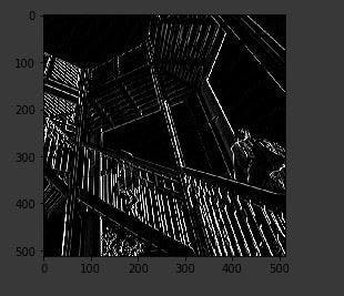
Matplotlib contains the code for drawing an image and it will render it right in the browser with Colab. Here, we can see the ascent image from SciPy. Next up, we’ll take a copy of the image, and we’ll add it with our homemade convolutions, and we’ll create variables to keep track of the x and y dimensions of the image. So we can see here that it’s a 512 by 512 image. So now, let’s create a convolution as a three by three array. We’ll load it with values that are pretty good for detecting sharp edges first. Here’s where we’ll create the convolution.

We then iterate over the image, leaving a one pixel margin. You’ll see that the loop starts at one and not zero, and it ends at size x minus one and size y minus one. In the loop, it will then calculate the convolution value by looking at the pixel and its neighbors, and then by multiplying them out by the values determined by the filter, before finally summing it all up.

Vertical line filter

Let’s run it. It takes just a few seconds, so when it’s done, let’s draw the results. We can see that only certain features made it through the filter. I’ve provided a couple more filters, so let’s try them. This first one is really great at spotting vertical lines. So when I run it, and plot the results, we can see that the vertical lines in the image made it through. It’s really cool because they’re not just straight up and down, they are vertical in perspective within the perspective of the image itself. Similarly, this filter works well for horizontal lines. So when I run it, and then plot the results, we can see that a lot of the horizontal lines made it through. Now, let’s take a look at pooling, and in this case, Max pooling, which takes pixels in chunks of four and only passes through the biggest value. I run the code and then render the output. We can see that the features of the image are maintained, but look closely at the axes, and we can see that the size has been halved from the 500’s to the 250's.

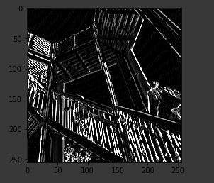With pooling

Excercise 3

Now you need to apply this to MNIST Handwrting recognition we will revisit that from last blog post. You need to improve MNIST to 99.8% accuracy or more using only a single convolutional layer and a single MaxPooling 2D. You should stop training once the accuracy goes above this amount. It should happen in less than 20 epochs, so it’s ok to hard code the number of epochs for training, but your training must end once it hits the above metric. If it doesn’t, then you’ll need to redesign your layers.

When 99.8% accuracy has been hit, you should print out the string “Reached 99.8% accuracy so cancelling training!”. Yes this is just optional (You can also print out something like “I’m getting bored and won’t train any more” 🤣)

The question notebook is available — here

My Solution

Wonderful! 😃 , you just coded for a handwriting recognizer with a 99.8% accuracy (that’s good) in less than 20 epochs. Let explore my solution for this.

def train_mnist_conv():
    # Please write your code only where you are indicated.
    # please do not remove model fitting inline comments.

    # YOUR CODE STARTS HERE
    class myCallback(tf.keras.callbacks.Callback):
        def on_epoch_end(self, epoch, logs={}):
            if(logs.get('acc')>0.998):
                print("/n Reached 99.8% accuracy so cancelling training!")
                self.model.stop_training = True
    # YOUR CODE ENDS HERE

    mnist = tf.keras.datasets.mnist
    (training_images, training_labels), (test_images, test_labels) = mnist.load_data()
    # YOUR CODE STARTS HERE
    callbacks = myCallback()

    training_images=training_images.reshape(60000, 28, 28, 1)
    test_images=test_images.reshape(10000, 28, 28, 1)
    training_images = training_images / 255.0
    test_images = test_images / 255.0
    # YOUR CODE ENDS HERE

    model = tf.keras.models.Sequential([
            # YOUR CODE STARTS HERE
            tf.keras.layers.Conv2D(64, (3,3), activation='relu', input_shape=(28, 28, 1)),
            tf.keras.layers.MaxPooling2D(2, 2),
            tf.keras.layers.Flatten(),
            tf.keras.layers.Dense(256, activation='relu'),
            tf.keras.layers.Dense(10, activation='softmax')
            # YOUR CODE ENDS HERE
    ])

    model.compile(optimizer='adam', loss='sparse_categorical_crossentropy', metrics=['accuracy'])
    # model fitting
    history = model.fit(
        # YOUR CODE STARTS HERE
        training_images,
        training_labels,
        epochs = 20,
        callbacks=[callbacks]
        # YOUR CODE ENDS HERE
    )
    # model fitting
    return history.epoch, history.history['acc'][-1]

The callback class (This is the simplest)

class myCallback(tf.keras.callbacks.Callback):

def on_epoch_end(self, epoch, logs={}):

if(logs.get('acc')>0.998):

print("/n Reached 99.8% accuracy so cancelling training!")

self.model.stop_training = True

The main CNN code

training_images=training_images.reshape(60000, 28, 28, 1)
    test_images=test_images.reshape(10000, 28, 28, 1)
    training_images = training_images / 255.0
    test_images = test_images / 255.0
    # YOUR CODE ENDS HERE

model = tf.keras.models.Sequential([
            # YOUR CODE STARTS HERE
            tf.keras.layers.Conv2D(64, (3,3), activation='relu', input_shape=(28, 28, 1)),
            tf.keras.layers.MaxPooling2D(2, 2),
            tf.keras.layers.Flatten(),
            tf.keras.layers.Dense(256, activation='relu'),
            tf.keras.layers.Dense(10, activation='softmax')
            # YOUR CODE ENDS HERE
    ])

So, all you had to do was play around the code and get this done in just 7 epochs.

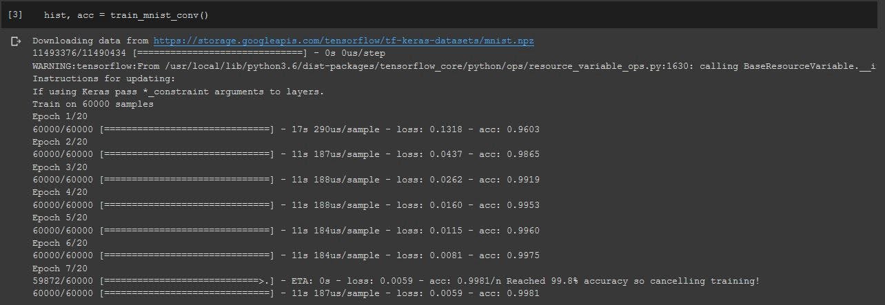My output

The solution notebook is available here

I hope this was helpful for you and you learned about visualizing CNNs and applying them on a real life data set, you also created a handwritten number recognizer all by yourself with a wonderful accuracy. That’s pretty good

About Me

Hi everyone I am Rishit Dagli

Twitter

Website

If you want to ask me some questions, report any mistake, suggest improvements, give feedback you are free to do so by emailing me at —