How to Build Better Machine Learning Models

Hello developers 👋. If you have built Deep Neural Networks before, you might know that it can involve a lot of experimentation.

In this article, I will share with you some useful tips and guidelines that you can use to better build better deep learning models. These tricks should make it a lot easier for you to develop a good network.

You can pick and choose which tips you use, as some will be more helpful for the projects you are working on. Not everything mentioned in this article will straight up improve your models’ performance.

A high-level approach for Hyperparameter tuning🕹️

One of the more painful things about training Deep Neural Networks is the large number of hyperparameters you have to deal with.

These could be your learning rate \( \alpha \), the discounting factor \( \rho \), and epsilon \( \epsilon \) if you are using the RMSprop optimizer (Hinton et al.) or the exponential decay rates \( \beta_1 \) and \( \beta_2 \) if you are using the Adam optimizer (Kingma et al.).

You also need to choose the number of layers in the network or the number of hidden units for the layers. You might be using learning rate schedulers and would want to configure those features and a lot more 😩! We definitely need ways to better organize our hyperparameter tuning process.

A common algorithm I tend to use to organize my hyperparameter search process is Random Search. Though there are other algorithms that might be better, I usually end up using it anyway.

Let’s say for the purpose of this example you want to tune two hyperparameters and you suspect that the optimal values for both would be somewhere between one and five.

The idea here is that instead of picking twenty-five values to try out like (1, 1) (1, 2) and so on systematically, it would be more effective to select twenty-five points at random.

Based on Lecture Notes of Andrew Ng

Here is a simple example with TensorFlow where I try to use Random Search on the Fashion MNIST Dataset for the learning rate and the number of units in the first Dense layer:

Here I suspect that an optimal number of units in the first Dense layer would be somewhere between 32 and 512, and my learning rate would be one of 1e-2, 1e-3, or 1e-4.

Consequently, as shown in this example, I set my minimum value for the number of units to be 32 and the maximum value to be 512 and have a step size of 32. Then, instead of hardcoding a value for the number of units, I specify a range to try out.

hp_units = hp.Int('units', min_value = 32, max_value = 512, step = 32)
model.add(tf.keras.layers.Dense(units = hp_units, activation = 'relu'))

We do the same for our learning rate, but our learning rate is simply one of 1e-2, 1e-3, or 1e-4 rather than a range.

hp_learning_rate = hp.Choice('learning_rate', values = [1e-2, 1e-3, 1e-4])
optimizer = tf.keras.optimizers.Adam(learning_rate = hp_learning_rate)

Finally, we perform Random Search and specify that among all the models we build, the model with the highest validation accuracy would be called the best model. Or simply that getting a good validation accuracy is the goal.

tuner = kt.RandomSearch(model_builder,
                        objective = 'val_accuracy', 
                        max_trials = 10,
                        directory = 'random_search_starter',
                        project_name = 'intro_to_kt') 

tuner.search(img_train, label_train, epochs = 10, validation_data = (img_test, label_test))

After doing so, I also want to retrieve the best model and the best hyperparameter choice. Though I would like to point out that using the get_best_models is usually considered a shortcut.

To get the best performance you should retrain your model with the best hyperparameters you get on the full dataset.

# Which was the best model?
best_model = tuner.get_best_models(1)[0]

# What were the best hyperparameters?
best_hyperparameters = tuner.get_best_hyperparameters(1)[0]

I won’t be talking about this code in detail in this article, but you can read about it in this article I wrote some time back if you want.

Use Mixed Precision Training for large networks🎨

The bigger your neural network is, the more accurate your results (in general). As model sizes grow, the memory and compute requirements for training these models also increase.

The idea with using Mixed Precision Training (NVIDIA, Micikevicius et al.) is to train deep neural networks using half-precision floating-point numbers which let you train large neural networks a lot faster with no or negligible decrease in the performance of the networks.

But, I’d like to point out that this technique should only be used for large models with more than 100 million parameters or so.

While mixed-precision would run on most hardware, it will only speed up models on recent NVIDIA GPUs (for example Tesla V100 and Tesla T4) and Cloud TPUs.

I want to give you an idea of the performance gains when using Mixed Precision. When I trained a ResNet model on my GCP Notebook instance (consisting of a Tesla V100) it was almost three times better in the training time and almost 1.5 times on a Cloud TPU instance with almost no difference in accuracy. The code to measure the above speed-ups was taken from this example.

To further increase your training throughput, you could also consider using a larger batch size — and since we are using float16 tensors you should not run out of memory.

It is also rather easy to implement Mixed Precision with TensorFlow. With TensorFlow you could easily use the tf.keras.mixed_precision Module that allows you to set up a data type policy (to use float16) and also apply loss scaling to prevent underflow.

Here is a minimalistic example of using Mixed Precision Training on a network:

In this example, we first set the dtype policy to be float16 which implies that all of our model layers will automatically use float16.

After doing so we build a model, but we override the data type for the last or the output layer to be float32 to prevent any numeric issues. Ideally, your output layers should be float32.

Note: I’ve built a model with so many units so we can see some difference in the training time with Mixed Precision Training since it works well for large models.

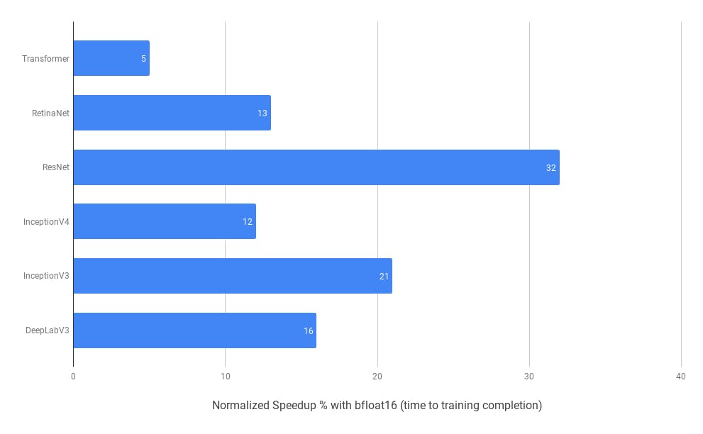
If you are looking for more inspiration to use Mixed Precision Training, here is an image demonstrating speedup for multiple models by Google Cloud on a TPU:

Speedups on a Cloud TPU

Use Grad Check for backpropagation✔️

In multiple scenarios, I have had to custom implement a neural network. And implementing backpropagation is typically the aspect that’s prone to mistakes and is also difficult to debug.

With incorrect backpropagation your model could learn something which might look reasonable, which makes it even more difficult to debug. So, how cool would it be if we could implement something which could allow us to debug our neural nets easily?

I often use Gradient Check when implementing backpropagation to help me debug it. The idea here is to approximate the gradients using a numerical approach. If it is close to the calculated gradients by the backpropagation algorithm, then you can be more confident that the backpropagation was implemented correctly.

As of now, you can use this expression in standard terms to get a vector which we will call \( d \theta [approx] \):

Calculate approx gradients

In case you are looking for the reasoning behind this, you can find more about it in this article I wrote.

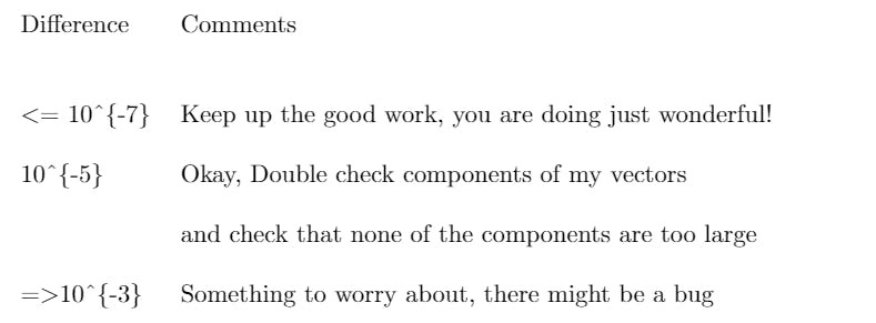
So, now we have two vectors \( d \theta [approx] \) and \( d \theta \) (calculated by backprop). And these should be almost equal to each other. You could simply compute the Euclidean distance between these two vectors and use this reference table to help you debug your nets:

A Reference table

Cache Datasets💾

Caching datasets is a simple idea but it’s not one I have seen used much. The idea here is to go over the dataset in its entirety and cache it either in a file or in memory (if it is a small dataset).

This should save you from performing some expensive CPU operations like file opening and data reading during every single epoch.

This does also means that your first epoch would comparatively take more time📉 since you would ideally be performing all operations like opening files and reading data in the first epoch and then caching them. But the subsequent epochs should be a lot faster since you would be using the cached data.

This definitely seems like a very simple to implement idea, right? Here is an example with TensorFlow showing how you can very easily cache datasets. It also shows the speedup 🚀 from implementing this idea. Find the complete code for the below example in this gist of mine.

A simple example of caching datasets and the speedup with it

How to tackle overfitting ⭐

When you’re working with neural networks, overfitting and underfitting might be two of the most common problems you face. This section talks about some common approaches that I use when tackling these problems.

You might know this, but high bias will cause you to miss a relationship between features and labels (underfitting) and high variance will cause the model to capture the noise and overfit to the training data.

I believe the most effective way to solve overfitting is to get more data — though you could also augment your data. A benefit of deep neural networks is that their performance improves as they are fed more and more data.

But in a lot of situations, it might be too expensive to get more data or it simply might not be possible to do so. In that case, let’s talk about a couple of other methods you could use to tackle overfitting.

Apart from getting more data or augmenting your data, you could also tackle overfitting either by changing the architecture of the network or by applying some modifications to the network’s weights. Let’s look at these two methods.

Changing the Model Architecture

A simple way to change the architecture such that it doesn’t overfit would be to use Random Search to stumble upon a good architecture. Or you could try pruning nodes from your model, essentially lowering the capacity of your model.

We already talked about Random Search, but in case you want to see an example of pruning you could take a look at the TensorFlow Model Optimization Pruning Guide.

Modifying Network Weights

In this section, we will see some methods I commonly use to prevent overfitting by modifying a network’s weights.

Weight Regularization

Iterating back on what we discussed, “simpler models are less likely to overfit than complex ones”. We try to keep a bar on the complexity of the network by forcing its weights only to take small values.

To do so we will add to our loss function a term that can penalize our model if it has large weights. Often \( L_1 \) and \( L_2 \) regularizations are used, the difference being:

• L1 — The penalty added is \( \propto \) to \( |weight coefficients| \)

• L2 — The penalty added is \( \propto \) to \( |weight coefficients|^2 \)

where \( |x| \) represents absolute values.

Do you notice the difference between L1 and L2, the square term? Due to this, L1 might push weights to be equal to zero whereas L2 would have weights tending to zero but not zero.

In case you are curious about exploring this further, this article goes deep into regularizations and might help.

This is also the exact reason why I tend to use L2 more than L1 regularization. Let’s see an example of this with TensorFlow.

Here I show some code to create a simple Dense layer with 3 units and the L2 regularization:

import tensorflow as tf
tf.keras.layers.Dense(3, kernel_regularizer = tf.keras.regularizers.L2(0.1))

To provide more clarity on what this does, as we discussed above this would add a term ( \( 0.1 \times weight coefficient value^2 \) ) to the loss function which works as a penalty to very big weights. Also, it is as easy as replacing L2 to L1 in the above code to implement L1 for your layer.

Dropouts

The first thing I do when I am building a model and face overfitting is try using dropouts (Srivastava et al.). The idea here is to randomly drop out or set to zero (ignore) x% of output features of the layer during training.

We do this to stop individual nodes from relying on the output of other nodes and prevent them from co-adapting from other nodes too much.

Dropouts are rather easy to implement with TensorFlow since they are available as layers. Here is an example of me trying to build a model to differentiate images of dogs and cats with Dropout to reduce overfitting:

model = tf.keras.models.Sequential([
    tf.keras.layers.Conv2D(32, (3,3), padding='same', activation='relu',input_shape=(IMG_HEIGHT, IMG_WIDTH ,3)),
    tf.keras.layers.MaxPooling2D(2,2),
    tf.keras.layers.Dropout(0.2),
    tf.keras.layers.Conv2D(128, (3,3), padding='same', activation='relu'),
    tf.keras.layers.MaxPooling2D(2,2),
    tf.keras.layers.Dropout(0.2),
    tf.keras.layers.Flatten(),
    tf.keras.layers.Dense(512, activation='relu'),
    tf.keras.layers.Dense(1, activation='sigmoid')
])

As you could see in the code above, you could directly use tf.keras.layers.dropout to implement the dropout, passing it the fraction of output features to ignore (here 20% of the output features).

Early stopping

Early stopping is another regularization method I often use. The idea here is to monitor the performance of the model at every epoch on a validation set and terminate the training when you meet some specified condition for the validation performance (like stop training when loss < 0.5)

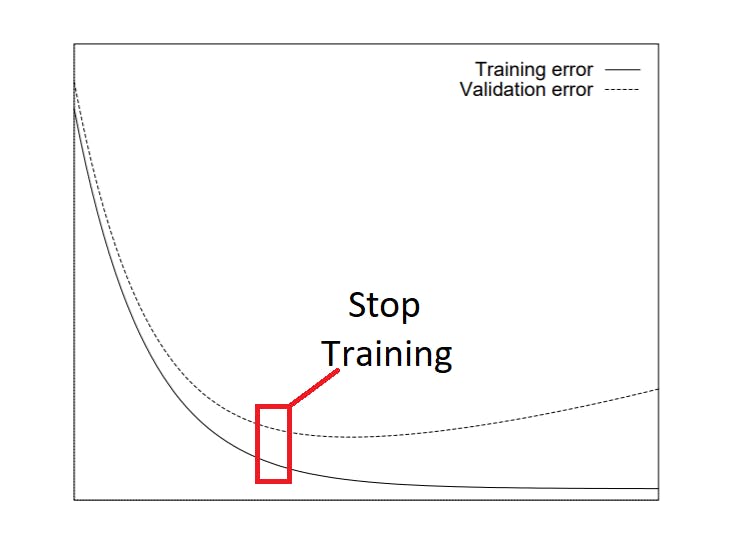
It turns out that the basic condition like we talked about above works like a charm if your training error and validation error look something like in this image. In this case, Early Stopping would just stop training when it reaches the red box (for demonstration) and would straight up prevent overfitting.

It (Early stopping) is such a simple and efficient regularization technique that Geoffrey Hinton called it a “beautiful free lunch”.

-Hands-On Machine Learning with Scikit-Learn and TensorFlow by Aurelien Geron

Adapted from Lutz Prechelt

However, for some cases, you would not end up with such straightforward choices for identifying the criterion or knowing when Early Stopping should stop training the model.

For the scope of this article, we will not be talking about more criteria here, but I would recommend that you check out “Early Stopping — But When, Lutz Prechelt” which I use a lot to help decide criteria.

Let’s see an example of Early Stopping in action with TensorFlow:

import tensorflow as tf

callback = tf.keras.callbacks.EarlyStopping(monitor='loss', patience=3)
model = tf.keras.models.Sequential([...])
model.compile(...)
model.fit(..., callbacks = [callback])

In the above example, we create an Early Stopping Callback and specify that we want to monitor our loss values. We also specify that it should stop training if it does not see noticeable improvements in loss values in 3 epochs. Finally, while training the model, we specify that it should use this callback.

Also, for the purpose of this example, I show a Sequential model — but this could work in the exact same manner with a model created with the functional API or sub-classed models, too.

Thank you for reading!

Thank you for sticking with me until the end. I hope you will benefit from this article and incorporate these tips in your own experiments.

I am excited to see if they help you improve the performance of your neural nets, too. If you have any feedback or suggestions for me please feel free to reach out to me on Twitter.