


Source: Cognitiveclass.ai
Table of contents
All the code used here is available in my GitHub repository here.
This is the third part of the series where I post about TensorFlow for Deep Learning and Machine Learning. In the earlier blog post you saw a basic Neural Network for Computer Vision. It did the job nicely, but it was a little naive in its approach. This time you’re going to improve on that using Convolutional Neural Networks(CNN). I believe in hands-on coding so we will have many exercises and demos which you can try yourself too. I would recommend you to play around with these exercises and change the hyper-parameters and experiment with the code. We will also be working with some real life data sets and apply the discussed algorithms on them too. If you have not read the previous article consider reading it once before you read this one here.
Introduction
I think it’s really cool that you’re already able to implement a neural network to do this fashion classification task. It’s just amazing that large data sets like this are readily available to you which makes it really easy to learn. And in this case we saw with just a few lines of code, we were able to build a DNN, deep neural net that allowed you to do this classification of clothing and we got reasonable accuracy with it but it was a little bit of a naive algorithm that we used, right? We’re looking at each and every pixel in every image, but maybe there are ways that we can make it better but maybe looking at features of what makes a shoe a shoe and what makes a handbag a handbag. What do you think? You might think something like if I have a shoelace in the picture it could be a shoe and if there is a handle it may be a handbag.
So, one of the ideas that make these neural networks work much better is to use convolutional neural networks, where instead of looking at every single pixel and say, getting the pixel values and then figuring out, “is this a shoe or is this a hand bag? I don’t know.” But instead you can look at a picture and say, “Ok, I see shoelaces and a sole.” Then, it’s probably shoe or say, “I see a handle and rectangular bag beneath that.” Probably a handbag. What’s really interesting about convolutions is that they sound very complicated but they’re actually quite straightforward. It is essentially just a filter that you pass over an image in the same way as if you’re doing some sharpening. If you have ever done image processing, it can spot features within the image just like we talked about. With the same paradigm of just data labels, we can let a neural network figure out for itself that it should look for shoe laces and soles or handles in bags and then just learn how to detect these things by itself. So we will also see how good or bad it works in comparison to our earlier approach for Fashion MNIST?
So, now we will know about convolutional neural networks and get to use it to build a much better fashion classifier.
What are Convolutions and Poolings
In the DNN approach, in just a couple of minutes, you’re able to train it to classify with pretty high accuracy on the training set, but a little less on the test set. Now, one of the things that you would have seen when you looked at the images is that there’s a lot of wasted space in each image. While there are only 784 pixels, it will be interesting to see if there was a way that we could condense the image down to the important features that distinguish what makes it a shoe, or a handbag, or a shirt. That’s where convolutions come in. So, what’s convolution at all?
 How filters work?
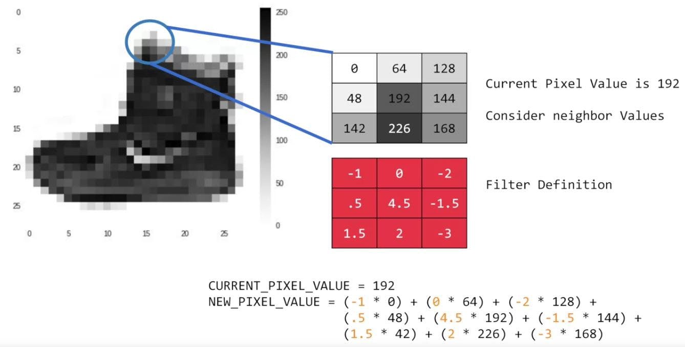
If you have ever done any kind of image processing, it usually involves having a filter and passing that filter over the image in order to change the underlying image. The process works a little bit like this. For every pixel, take its value, and take a look at the value of its neighbors. If our filter is three by three, then we can take a look at the immediate neighbor, so that you have a corresponding 3 by 3 grid. Then to get the new value for the pixel, we simply multiply each neighbor by the corresponding value in the filter. So, for example, in this case, our pixel has the value 192, and its upper left neighbor has the value 0. The upper left value and the filter is -1, so we multiply 0 by -1. Then we would do the same for the upper neighbor. Its value is 64 and the corresponding filter value was 0, so we’d multiply those out.
Repeat this for each neighbor and each corresponding filter value, and would then have the new pixel with the sum of each of the neighbor values multiplied by the corresponding filter value, and that’s a convolution. It’s really as simple as that. The idea here is that some convolutions will change the image in such a way that certain features in the image get emphasized.
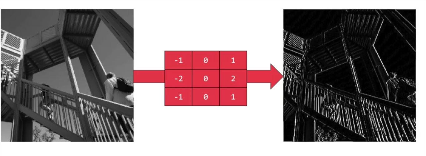
So, for example, if you look at this filter, then the vertical lines in the image really pop out. Don’t worry we will do a hands-on for this later.
 A filter which pops out vertical lines
With this filter, the horizontal lines pop out.
 A filter which pops out horizontal lines
Now, that’s a very basic introduction to what convolutions do, and when combined with something called pooling, they can become really powerful.
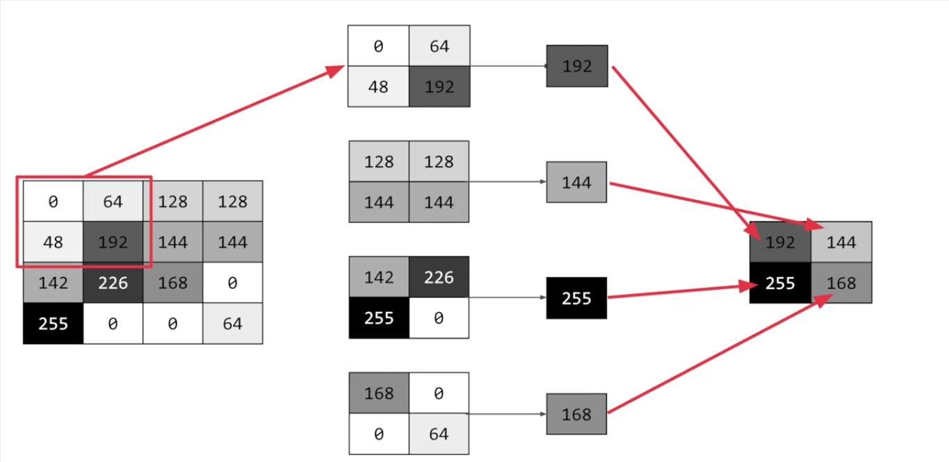
Now what’s pooling then? pooling is a way of compressing an image. A quick and easy way to do this, is to go over the image of 4 pixels at a time, that is, the current pixel and its neighbors underneath and to the right of it.
 a 4 x 4 pooling
Of these 4, pick the biggest value and keep just that. So, for example, you can see it here. My 16 pixels on the left are turned into the four pixels on the right, by looking at them in 2 by 2 grids and picking the biggest value. This will preserve the features that were highlighted by the convolution, while simultaneously quartering the size of the image. We have the horizontal and vertical axes too.
Coding for convolutions and max pooling
These layers are available as
Conv2D and
in TensorFlow.
We don’t have to do all the math for filtering and compressing, we simply define convolutional and pooling layers to do the job for us.
So here’s our code from the earlier example, where we defined out a neural network to have an input layer in the shape of our data, and output layer in the shape of the number of categories we’re trying to define, and a hidden layer in the middle. The Flatten takes our square 28 by 28 images and turns them into a one dimensional array.
model = tf.keras.models.Sequential([

  tf.keras.layers.Flatten(input_shape=(28, 28)),
  tf.keras.layers.Dense(128, activation = tf.nn.relu,
  tf.keras.layers.Dense(10, activation = tf.nn.softmax

])
To add convolutions to this, you use code like this.
model = tf.keras.models.Sequential([

  tf.keras.layers.Conv2D(64, (3,3), activation='relu',     input_shape=(28, 28, 1)),

  tf.keras.layers.MaxPooling2D(2, 2),

  tf.keras.layers.Conv2D(64, (3,3), activation='relu'),

  tf.keras.layers.MaxPooling2D(2,2),

  tf.keras.layers.Flatten(),

  tf.keras.layers.Dense(128, activation='relu'),

  tf.keras.layers.Dense(10, activation='softmax')

])
You’ll see that the last three lines are the same, the Flatten, the Dense hidden layer with 128 neurons, and the Dense output layer with 10 neurons. What’s different is what has been added on top of this. Let’s take a look at this, line by line.
tf.keras.layers.Conv2D(64, (3,3), activation='relu', input_shape=(28, 28, 1))
Here we’re specifying the first convolution. We’re asking keras to generate 64 filters for us. These filters are 3 by 3, their activation is relu, which means the negative values will be thrown way, and finally the input shape is as before, the 28 by 28. That extra 1 just means that we are tallying using a single byte for color depth. As we saw before our image is our gray scale, so we just use one byte. Now, of course, you might wonder what the 64 filters are. It’s a little beyond the scope of this blog to define them, but they for now you can understand that they are not random. They start with a set of known good filters in a similar way to the pattern fitting that you saw earlier, and the ones that work from that set are learned over time.
tf.keras.layers.MaxPooling2D(2, 2)
This next line of code will then create a pooling layer. It’s max-pooling because we’re going to take the maximum value. We’re saying it’s a two-by-two pool, so for every four pixels, the biggest one will survive as shown earlier. We then add another convolutional layer, and another max-pooling layer so that the network can learn another set of convolutions on top of the existing one, and then again, pool to reduce the size. So, by the time the image gets to the flatten to go into the dense layers, it’s already much smaller. It’s being quartered, and then quartered again. So, its content has been greatly simplified, the goal being that the convolutions will filter it to the features that determine the output.
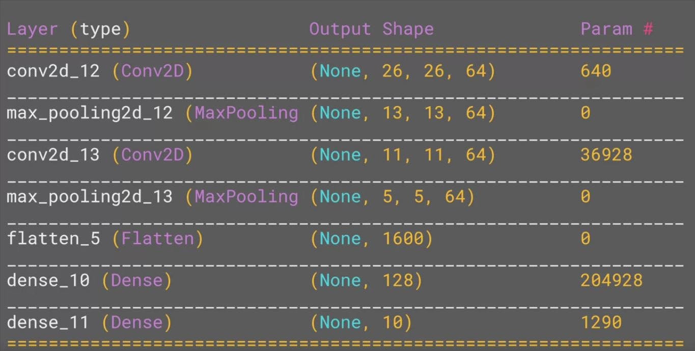
A really useful method on the model is the model.summary method. This allows you to inspect the layers of the model, and see the journey of the image through the convolutions, and here is the output.
 Output of model.summary
It’s a nice table showing us the layers, and some details about them including the output shape. It’s important to keep an eye on the output shape column. When you first look at this, it can be a little bit confusing and feel like a bug. After all, isn’t the data 28 by 28, so why is the output, 26 by 26? The key to this is remembering that the filter is a 3 by 3 filter. Consider what happens when you start scanning through an image starting on the top left. So, you can’t calculate the filter for the pixel in the top left, because it doesn’t have any neighbors above it or to its left. In a similar fashion, the next pixel to the right won’t work either because it doesn’t have any neighbors above it. So, logically, the first pixel that you can do calculations on is this one, because this one of course has all 8 neighbors that a three by 3 filter needs. This when you think about it, means that you can’t use a 1 pixel margin all around the image, so the output of the convolution will be 2 pixels smaller on x, and 2 pixels smaller on y. If your filter is five-by-five for similar reasons, your output will be four smaller on x, and four smaller on y. So, that’s y with a three by three filter, our output from the 28 by 28 image, is now 26 by 26, we’ve removed that one pixel on x and y, and each of the borders.
So, now our output gets reduced from 26 by 26, to 13 by 13. The convolutions will then operate on that, and of course, we lose the 1 pixel margin as before, so we’re down to 11 by 11, add another 2 by 2 max-pooling to have this rounding down, and went down, down to 5 by 5 images. So, now our dense neural network is the same as before, but it’s being fed with five-by-five images instead of 28 by 28 ones.
But remember, it’s not just one compressed 5 by 5 image instead of the original 28 by 28, there are a number of convolutions per image that we specified, in this case 64. So, there are 64 new images of 5 by 5 that had been fed in. Flatten that out and you have 25 pixels times 64, which is 1600. So, you can see that the new flattened layer has 1,600 elements in it, as opposed to the 784 that you had previously. This number is impacted by the parameters that you set when defining the convolutional 2D layers. Later when you experiment, you’ll see what the impact of setting what other values for the number of convolutions will be, and in particular, you can see what happens when you’re feeding less than 784 over all pixels in. Training should be faster, but is there a sweet spot where it’s more accurate?
To know more about this, implement this on a real life data set and even visualize the journey of an image through a CNN please head on to the next blog.
About Me
Hi everyone I am Rishit Dagli
If you want to ask me some questions, report any mistake, suggest improvements, give feedback you are free to do so by emailing me at —