Characterizing the sample complexity of different machine learning tasks is one of the central questions in statistical learning theory. For example, the classic Vapnik-Chervonenkis theory ^devroye1996vapnik characterizes the sample complexity of binary classification. Despite this early progress, the sample complexity of many important learning tasks - including density estimation and learning under adversarial perturbations - are not yet resolved. This blog reviews the less conventional approach of using compression schemes for proving sample complexity upper bounds, with specific applications in learning under adversarial perturbations and learning Gaussian mixture models. This article is mostly about what I learned from the paper, "Adversarially Robust Learning with Tolerance" ^ashtiani23a.

Standard Notation

I will first review some standard notation:

• \(Z\): domain set

• \(D_Z\): distribution over \(Z\)

• \(S\): i.i.d sample from \(D_Z\)

• \(H\): class of models/hypotheses

• \(L(D_Z,H) \to \mathbb{R}\): loss/ error function

• \(OPT=inf_{h \in H} L(D_z,h)\): best achievable

• \(A_{Z,H}: Z^* \to H\): learner

Density Estimation

Our goal for the task of density estimation is that for every \(DZ\), \(A{Z,H}(S)\) we want it to be comparable to \(OPT\) with high probability.

We take the example of density estimation, in this case, \(L(DZ, h) = d{TV} (Dz, h)\). Now, \(A{Z,H}\) probably approximately correct learns \(H\) with \(m(\epsilon, \delta)\) samples if for all \(D_Z\) and for all \(\epsilon\) with a \(\delta \in ( 0,1 )\). Now if \(S \sim D_Z^{m(\epsilon, \delta)}\) then:

$$\underset{S}{\mathrm{Pr}} [L(DZ, A{Z,H}(S)) > \epsilon + C \cdot OPT] < \delta$$

Now if we take the example of \(C=2\), let \(H\) be the set of all Gaussians in \(\mathbb{R}^d\) then:

$$m(\epsilon, \delta) = O \left( \frac{d^2 + \log 1/\delta}{\epsilon^2} \right)$$

We will now modify the above equation. Now, \(A_{Z,H}\) probably approximately correct learns \(H\) with \(m(\epsilon)\) samples if for all \(D_Z\) and for all \(\epsilon \in ( 0,1 )\). Now if \(S \sim D_Z^{m(\epsilon)}\) then:

$$\underset{S}{\mathrm{Pr}} [L(DZ, A{Z,H}(S)) > \epsilon + C \cdot OPT] < 0.01$$

For the example of \(C=2\), let \(H\) be the set of all Gaussians in \(\mathbb{R}^d\) then:

$$m(\epsilon, \delta) = O \left( \frac{d^2}{\epsilon^2} \right)$$

Binary Classification (with adv. perturbations)

For the example of binary classification, we have \(Z = X \times { 0, 1 }\) and \(h\) is some model which maps from \(h: X \to { 0, 1 }\).

We also have \(l(h,x,y) = 1 {h(x) \neq y}\) and then we will have the \(L\) be \(L(DZ,h) = E{(x,y) \sim D_Z} l(h,x,y)\).

Now, \(A_{Z,H}\) probably approximately correct learns \(H\) with \(m(\epsilon)\) samples if for all \(D_Z\) and for all \(\epsilon \in ( 0,1 )\). Now if \(S \sim D_Z^{m(\epsilon)}\) then:

$$\underset{S}{\mathrm{Pr}} [L(DZ, A{Z,H}(S)) > \epsilon + C \cdot OPT] < 0.01$$

Now \(H\) is the set of all half spaces in \(\mathbb{R}^d\) then:

$$m(\epsilon) = O \left( \frac{d}{\epsilon^2} \right)$$

For the example of binary classification, we have \(Z = X \times { 0, 1 }\) and \(h\) is some model which maps from \(h: X \to { 0, 1 }\).

We also have \(l^U(h,x,y) =\) adversarial perturbations and then we will have the \(L^U\) be \(L^U(DZ,h) = E{(x,y) \sim D_Z} l^U(h,x,y)\).

Now, \(A_{Z,H}\) probably approximately correct learns \(H\) with \(m(\epsilon)\) samples if for all \(D_Z\) and for all \(\epsilon \in ( 0,1 )\). Now if \(S \sim D_Z^{m(\epsilon)}\) then:

$$\underset{S}{\mathrm{Pr}} [L^U(DZ, A{Z,H}(S)) \epsilon + OPT] < 0.01$$

Now, consider the following \(H_1\) and \(H_2\):

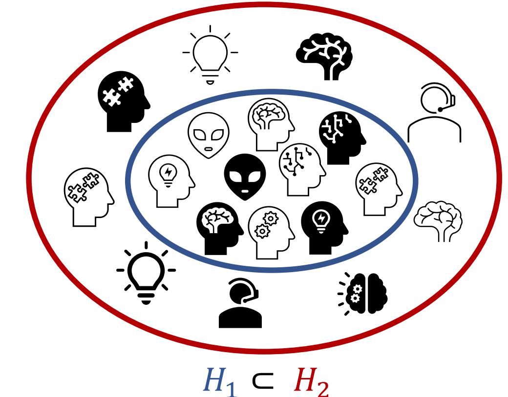
Here \(H_2\) is richer which can make it contain better models as well as harder to learn. We can characterize the sample complexity of learning \(H\) using Binary classification, with Binary classification with adversarial perturbations or with Density estimation.

In the case of binary classification the VC-dimension quantifies complexity:

$$m ( \epsilon ) = \Theta \left( \frac{VC(H)}{\epsilon^2} \right)$$

The upper bound here is achieved using simple ERM

$$L(S,h) = \frac{1}{|S|} \sum_{(x,y)\in S} l(h,x,y)$$

$$h = argmin_{h \in H} L(S,h)$$

And then for uniform convergence:

$$sup_{h \in H} |L(S,h) - L(D_z,h)| = O \left( \sqrt{\frac{VC(H)}{|S|}} \right) w.p. > 0.99$$

We now introduce sample compression as an alternative.

Sample Compression

The idea is to try and answer how should we go about compressing a given training set? In classic information theory, we would compress it into a few bits. In the case of sample compression, we want to try to compress it into a few samples.

If we just take the simple example of linear classification Number of required bits is unbounded (depends on the sample).

It has already been shown by ^littlestone1986relating that Compressibility \(\implies\) Learnability

$$m(\epsilon)=\tilde{O} \left( \frac{k}{\epsilon^2} \right)$$

It has also been shown by ^moran2016sample, Compressibility \(\impliedby\) Learnability

$$k = 2^{O(VC)}$$

Compression Conjecture:

\(k = \Theta(VC)\)

Sample Compression can be very helpful by:

• being simpler and more intuitive

• being more generic. It can work even if uniform convergence fails! Can show optimal SVM bound and we can also perform compression for learning under Adversarial Perturbations.

Typical classifiers are often:

• Sensitive to "adversarial" perturbations, even when the noise is "imperceptible"

• Vulnerable to malicious attacks

• Ignore the "invariance" or domain-knowledge

In the case of classification with adversarial perturbations we had \(l^{0/1}(h,x,y) = 1 {h(x) \neq y}\) and \(l^U(h,x,y) = sup_{\bar{x} \in U(x)} l^{0/1}(h,\bar{x},y)\)

and then we will have the \(L^U\) be \(L^U(DZ,h) = E{(x,y) \sim D_Z} l^U(h,x,y)\).

Now, \(A_{Z,H}\) probably approximately correct learns \(H\) with \(m(\epsilon)\) samples if for all \(D_Z\) and for all \(\epsilon \in ( 0,1 )\). Now if \(S \sim D_Z^{m(\epsilon)}\) then:

$$\underset{S}{\mathrm{Pr}} [L^U(DZ, A{Z,H}(S)) \epsilon + OPT] < 0.01$$

However one of the problems with this is if the robust ERM works for all \(H\)

$$L(S,h) = \frac{1}{|S|} \sum_{(x,y)\in S} l(h,x,y)$$

$$h = argmin_{h \in H} L(S,h)$$

The robust ERM would not work for all \(H\), uniform convergence can fail,

$$sup_{h \in H} |L^U(S,h) - L^U(D_z, h)|$$

can be unbounded.

We can say that any "proper learner" (outputs from \(H\)) can fail.

In a compression-based method the decoder should recover the labels of the training set and their neighbors and then compress the inflates set:

$$k = 2^{O(VC)}$$

So,

$$m^U(\epsilon) = O \left( \frac{2^{VC(H)}}{\epsilon^2} \right)$$

There is an exponential dependence on \(VC(H)\).

^ashtiani23a introduced tolerant adversarial learning \(A_{Z,H}\) PAC learns \(H\) with \(m(\epsilon)\) samples

if \(\forall D_Z\), \(\forall \epsilon \in (0,1)\), if \(S \simeq D_Z^{m(\epsilon)}\) then

$$Pr_S[L^U(DZ,A{Z,H}(S)) > \epsilon + inf_{h \in H} L^V(DZ,A{Z,H}(S))] < 0.01$$

And,

$$m^{U,V}(\epsilon) = \tilde{O} \left( \frac{VC(H)d\log(1+\frac{1}{\gamma})}{\epsilon ^2} \right)$$

The trick is to avoid compressing an infinite set and now our new goal is that the decoder should only recover labels of things in \(U(x)\).

To do so we can define a noisy empirical distribution (using \(V(x)\)) and then use boosting to achieve a super small error with respect to this distribution. And then, we encode the classifier using the samples used to train weak learners and the decoder smooths out the hypotheses.

It is interesting to think of Why do we need tolerance? There do exist some other ways to relax the problem and avoid \(2^{O(VC)}\)

• bounded adversary

• Limited black-box query access to the hypothesis

• Related to the certification problem

This is also observable in the density estimation example.

Gaussian Mixture Models

Gaussian mixture Models are very popular in practice and are one of the most basic universal density approximators. These are also the building blocks for more sophisticated density classes and can think of them as multi-modal versions of Gaussians.

$$f(x) = w_1N(x|\mu_1,\sum 1)+w_2N(x|\mu_2,\sum 2)+w_3N(x|\mu_3,\sum 3)$$

We say \(F\) is Gaussian Mixture Model with \(k\) components in \(\mathbb{R}^d\). And we want to ask how many samples is needed to recover \(f \in F\) within \(L_1\) error \(\epsilon\).

The number of samples \(\simeq m(d,k,\epsilon)\).

To learn single Gaussian in \(\mathbb{R}^d\) then

$$O \left( \frac{d^2}{\epsilon^2} \right) = O \left( \frac{# params}{\epsilon^2} \right)$$

samples are sufficient (and necessary).

Now if we have \(k\) Gaussian in \(\mathbb{R}^d\) then we want to know if

$$O \left( \frac{kd^2}{\epsilon^2} \right) = O \left( \frac{ \text{number of params}}{\epsilon^2} \right)$$

samples are sufficient?

There have been some results on learning Gaussian Mixture Models.

Let us take the example of this graph. For a moment look at this as a binary classification problem. The decision boundary has a simple quadratic form!

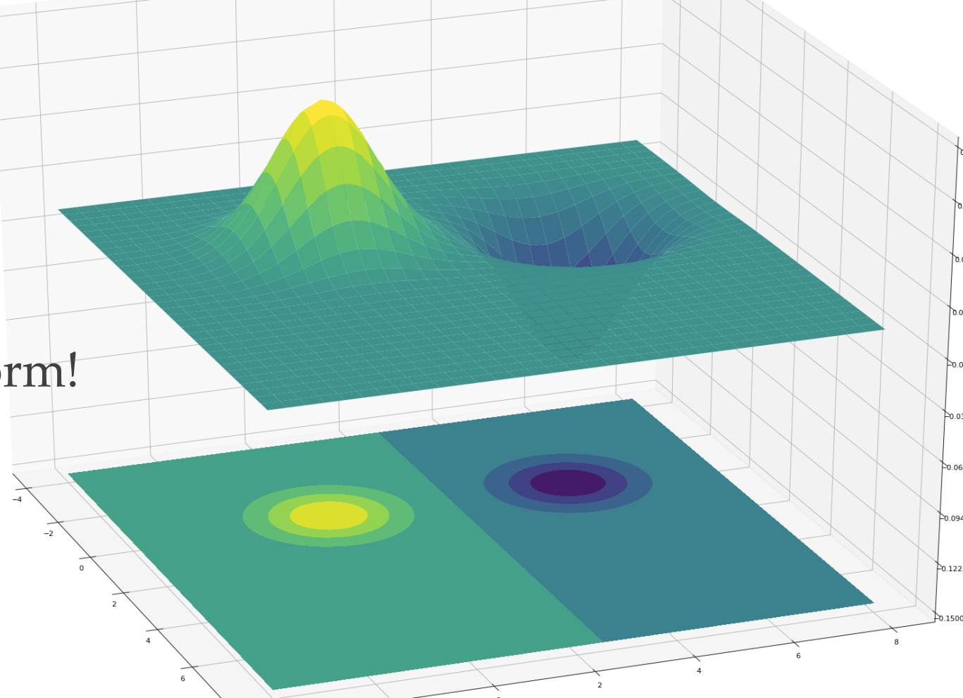
$$VC-dim=O(D^2)$$

Here "Sample compression" does not make sense as there are no "labels".

Compression Framework

We have \(F\) which is a class of distributions (e.g. Gaussians) and we have. If A sends \(t\) points from \(m\) points and B approximates \(D\) then we say \(F\) admits \((t,m)\)-compression.

Theorem:

If \(F\) has a compression scheme of size \((t,m)\) then sample complexity of learning \(F\) is

$$\tilde{O} \left( \frac{t}{\epsilon^2} + m \right)$$

\(\tilde{O}(\cdot)\) hides polylog factors.

Small compression schemes imply sample-efficient algorithms.

Theorem:

If \(F\) has a compression scheme of size \((t, m)\) then \(k\) mixtures of \(F\) admits \((kt,km)\) compression.

Distribution compression schemes extend to mixture classes automatically! So for the case of GMMs in \(\mathbb{R}^d\) it is enough to come up with a good compression scheme for a single Gaussian!

For learning mixtures of Gaussians, the encoding center and axes of ellipsoid is sufficient to recover \(N(\mu,\Sigma)\). This admits \(\tilde{O}(d^2,\frac{1}{\epsilon})\) compression! The technical challenge is encoding the \(d\) eigenvectors "accurately" using only \(d^2\) points.

\( \frac{\sigma{max}}{\sigma{min}} \) can be large which is a technical challenge.

Conclusion

• Compression is simple, intuitive, generic

• Compression relies heavily on a few points

  • But still can give "robust" methods

  • Agnostic sample compression

  • Robust target compression

• Target compression is quite general

  • Reduces the problem to learning from finite classes

  • Does it characterize learning?