Source: Cognitiveclass.ai
Table of contents
All the code used here is available at the GitHub repository here.
This is the second part of the series where I post about TensorFlow for Deep Learning and Machine Learning. In the earlier blog post, you learned all about how Machine Learning and Deep Learning is a new programming paradigm. This time you’re going to take that to the next level by beginning to solve problems of computer vision with just a few lines of code! I believe in hands-on coding so we will have many exercises and demos which you can try yourself too. I would recommend you to play around with these exercises and change the hyper-parameters and experiment with the code. We will also be working with some real-life data sets and apply the discussed algorithms to them too. If you have not read the previous article consider reading it once before you read this one here.
Introduction
So fitting straight lines seems like the “Hello, world” most basic implementation learning algorithm. But one of the most amazing things about machine learning is that, that core of the idea of fitting the x and yrelationship is what lets us do amazing things like, have computers look at the picture and do activity recognition, or look at the picture and tell us, is this a dress, or a pair of pants, or a pair of shoes; really hard for humans, and amazing that computers can now use this to do these things as well. Right, like computer vision is a really hard problem to solve, right? Because you’re saying like dress or shoes. It’s like how would I write rules for that? How would I say, if this pixel then it’s a shoe, if that pixel then its a dress? It’s really hard to do, so the labeled samples are the right way to go. One of the non-intuitive things about vision is that it’s so easy for a person to look at you and say, you’re wearing a shirt, it’s so hard for a computer to figure it out.
Because it’s so easy for humans to recognize objects, it’s almost difficult to understand why this is a complicated thing for a computer to do. What the computer has to do is look at all numbers, all the pixel brightness value, saying look at all of these numbers saying, these numbers correspond to a black shirt, and it’s amazing that with machine and deep learning computers are getting really good at this.
Computer Vision
Computer vision is the field of having a computer understand and label what is present in an image. When you look at this image below, you can interpret what a shirt is or what a shoe is, but how would you program for that? If an extraterrestrial who had never seen clothing walked into the room with you, how would you explain the shoes to him? It’s really difficult, if not impossible to do right? And it’s the same problem with computer vision. So one way to solve that is to use lots of pictures of clothing and tell the computer what that’s a picture of and then have the computer figure out the patterns that give you the difference between a shoe, and a shirt, and a handbag, and a coat.
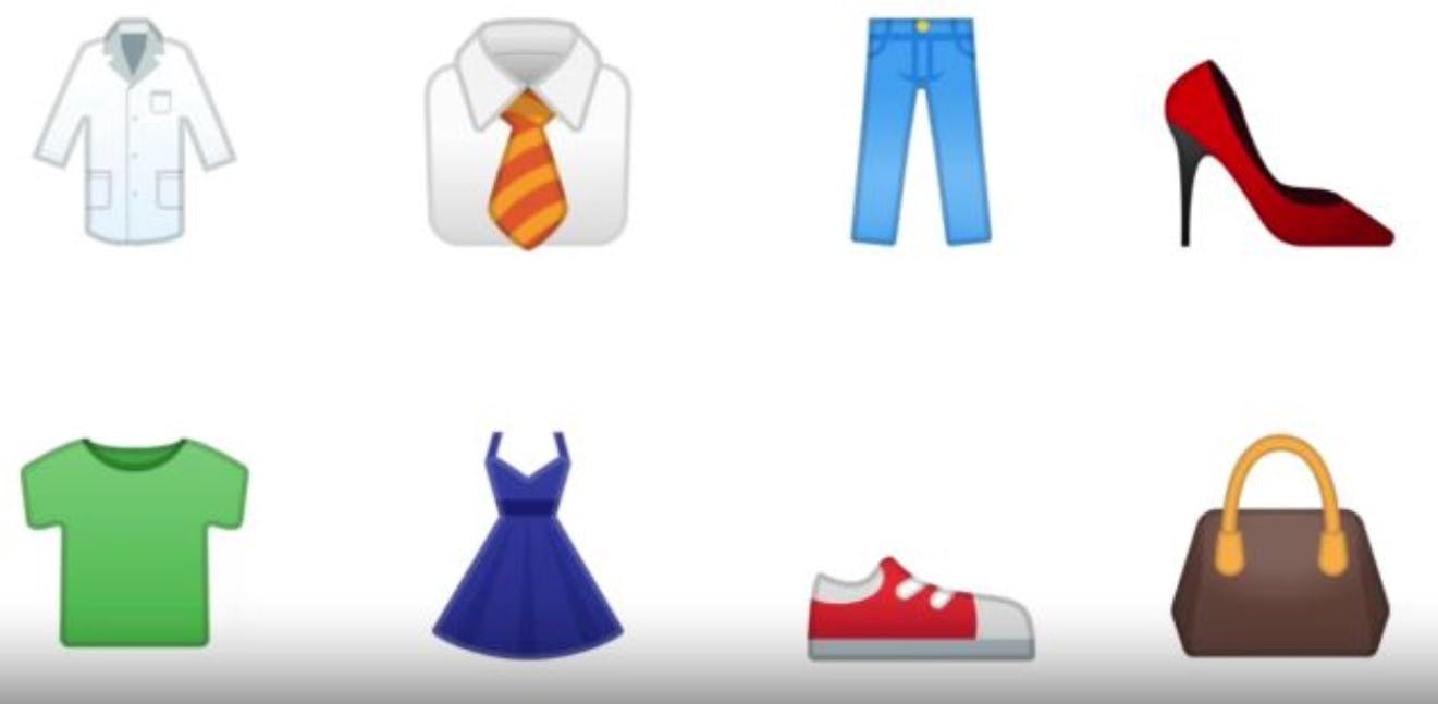 Image example
Let’s Get started
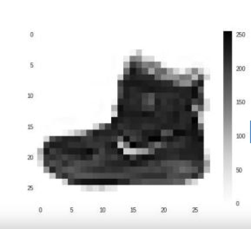
Fortunately, there’s a data set called Fashion MNIST (not to be confused with handwriting MNIST data set- that’s your exercise) which gives a 70,000 images spread across 10 different items of clothing. These images have been scaled down to 28 by 28 pixels. Now usually, the smaller the better because the computer has less processing to do. But of course, you need to retain enough information to be sure that the features and the object can still be distinguished. If you look at the image you can still tell the difference between shirts, shoes, and handbags. So this size does seem to be ideal, and it makes it great for training a neural network. The images are also in grayscale, so the amount of information is also reduced. Each pixel can be represented in values from zero to 255 and so it’s only one byte per pixel. With 28 by 28 pixels in an image, only 784 bytes are needed to store the entire image. Despite that, we can still see what’s in the image below, and in this case, it’s an ankle boot, right?
 An image from the data set
You can know more about the fashion MNIST data set at this GitHub repository here. You can also download the data set from here.
So what will handling this look like in code? In the previous blog post, you learned about TensorFlow and Keras, and how to define a simple neural network with them. Here, you are going to use them to go a little deeper but the overall API should look familiar. The one big difference will be in the data. The last time you had just your six pairs of numbers, so you could hard code it. This time you have to load 70,000 images off the disk, so there will be a bit of code to handle that. Fortunately, it’s still quite simple because Fashion MNIST is available as a data set with an API call in TensorFlow.
fashion_mnist = keras.datasets.fashion_mnist
(train_images, train_labels), (test_images, test_labels) =              fashion_mnist.load_data()
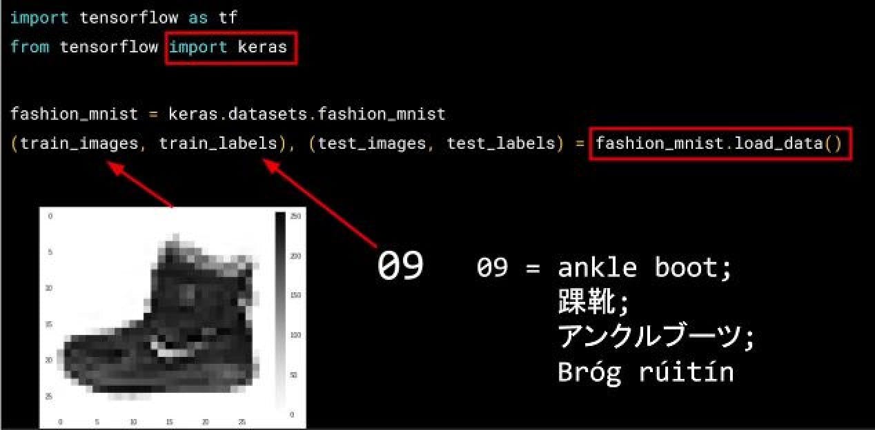
Consider the code fashion_mnist.load_data() . What we are doing here is creating an object of type MNIST and loading it from the Keras database. Now, on this class we are running a method called load_data() which will return four lists to us train_images , train_labels , test_images and test_labels . Now, what are these you might wonder? So, when building a neural network like this, it's a nice strategy to use some of your data to train the neural network and similar data that the model hasn't yet seen to test how good it is at recognizing the images. So in the Fashion MNIST data set, 60,000 of the 70,000 images are used to train the network, and then 10,000 images, one that it hasn't previously seen, can be used to test just how good or how bad the model is performing. So this code will give you those sets.
 An image from the data set and the code used
So for example, the training data will contain images like this one, and a label that describes the image like this. While this image is an ankle boot, the label describing it is number nine. Now, why do you think that is? There are two main reasons. First, of course, is that computers do better with numbers than they do with texts. Second, importantly, is that this is something that can help us reduce bias. If we labeled it as an ankle boot, we would be of course biased towards English speakers. But with it being a numeric label, we can then refer to it in our appropriate language be it English, Hindi, German, Mandarin, or here, even Irish. You can learn more about bias and techniques to avoid it here.
Coding a Neural Network for this
Okay. So now we will look at the code for the neural network definition. Remember last time we had a sequential with just one layer in it. Now we have three layers.
model = keras.Sequential([

    keras.layers.Flatten(input_shape = (28, 28)),
    keras.layers.Dense(128, activation = tf.nn.relu),
    keras.layers.Dense(10, activation = tf.nn.softmax)


])
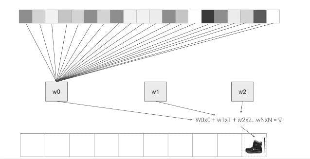
The important things to look at are the first and the last layers. The last layer has 10 neurons in it because we have ten classes of clothing in the data set. They should always match. The first layer is a Flatten layer with the input shaping 28 by 28. Now, if you remember our images are 28 by 28, so we’re specifying that this is the shape that we should expect the data to be in. Flatten takes this 28 by 28 square and turns it into a simple linear array. The interesting stuff happens in the middle layer, sometimes also called a hidden layer. This is 128 neurons in it, and I’d like you to think about these as variables in a function. Maybe call them x1, x2 x3, etc. Now, there exists a rule that incorporates all of these that turns the 784 values of an ankle boot into the value nine, and similar for all of the other 70,000.
 A neural net layer
So, what the neural net does is figure out w0 , w1 , w2 … w n such that (x1 * w1) + (x2 * w2) ... (x128 * w128) = y
You’ll see that it’s doing something very, very similar to what we did earlier when we figured out y = 2x — 1. In that case, the two was the weight of x. So, I’m saying y = w1 * x1, etc. The important thing now is to get the code working, so you can see a classification scenario for yourself. You can also tune the neural network by adding, removing, and changing layer size to see the impact.
As we discussed earlier to finish this example and writing the complete code we will use Tensor Flow 2.x, before that we will explore few Google Colaboratory tips as that is what you might be using. However, you can also use Jupyter Notebooks preferably in your local environment.
Colab Tips (OPTIONAL)
- Map your Google Drive
On Colab notebooks you can access your Google Drive as a network mapped drive in the Colab VM runtime.
# You can access to your Drive files using this path "/content
# /gdrive/My Drive/"

from google.colab import drive
drive.mount('/content/gdrive')
- Work with your files transparently on your computer
You can sync a Google Drive folder on your computer. Along with the previous tip, your local files will be available locally in your Colab notebook.
- Clean your root folder on Google Drive
There are some resources from Google that explains that having a lot of files in your root folder can affect the process of mapping the unit. If you have a lot of files in your root folder on Drive, create a new folder and move all of them there. I suppose that having a lot of folders on the root folder will have a similar impact.
- Hardware acceleration
For some applications, you might need a hardware accelerator like a GPU or a TPU. Let’s say you are building a CNN or so 1 epoch might be 90–100 seconds on a CPU but just 5–6 seconds on a GPU and in milliseconds on a TPU. So, this is definitely helpful. You can go to-
Runtime > Change Runtime Type > Select your hardware accelerator
- A fun feature
This is called power level. Power level is an April fools joke feature that adds sparks and combos to cell editing. Access using-
Tools > Settings > Miscellaneous > Select Power
 Example of high power
Walkthrough the notebook
The notebook is available here. If you are using a local development environment, download this notebook; if you are using Colab click the open in colab button. We will also see some exercises in this notebook.
try:
  # %tensorflow_version only exists in Colab.
  %tensorflow_version 2.x
except Exception:
  pass

import tensorflow as tf
First, we use the above code to import TensorFlow 2.x, If you are using a local development environment you do not need lines 1–5.
Then, as discussed we use this code to get the data set.
fashion_mnist = keras.datasets.fashion_mnist
(train_images, train_labels), (test_images, test_labels) =              fashion_mnist.load_data()
We will now use matplotlib to view a sample image from the dataset.
import matplotlib.pyplot as plt
plt.imshow(training_images[0])
You can change the 0 to other values to get other images as you might have guessed. You’ll notice that all of the values in the number are between 0 and 255. If we are training a neural network, for various reasons it’s easier if we treat all values as between 0 and 1, a process called ‘normalizing’ and fortunately, in Python, it’s easy to normalize a list like this without looping. You do it like this:
training_images  = training_images / 255.0
test_images = test_images / 255.0
Now in the next code block in the notebook we have defines the same neural net we earlier discussed. Ok, so you might have noticed a change in we use softmax function. Softmax takes a set of values, and effectively picks the biggest one, so, for example, if the output of the last layer looks like [0.1, 0.1, 0.05, 0.1, 9.5, 0.1, 0.05, 0.05, 0.05], it saves you from fishing through it looking for the biggest value, and turns it into [0,0,0,0,1,0,0,0,0] — The goal is to save a lot of coding!
We can then try to fit the training images to the training labels. We’ll just do it for 10 epochs to be quick. We spend about 50 seconds training it over five epochs and we end up with a loss of about 0.205. That means it’s pretty accurate in guessing the relationship between the images and their labels. That’s not great, but considering it was done in just 50 seconds with a very basic neural network, it’s not bad either. But a better measure of performance can be seen by trying the test data. These are images that the network has not yet seen. You would expect performance to be worse, but if it’s much worse, you have a problem. As you can see, it’s about 0.32 loss, meaning it’s a little bit less accurate on the test set. It’s not great either, but we know we’re doing something right.
I have some questions and exercises for you 8 in all and I recommend you to go through all of them, you will also be exploring the same example with more neurons and things like that. So have fun coding.
You just made a complete fashion MNIST algorithm that can predict with pretty good accuracy the images of fashion items.
Callbacks (Very important)
How can I stop training when I reach a point that I want to be at? What do I always have to hard code it to go for a certain number of epochs? So in every epoch, you can callback to a code function, having checked the metrics. If they’re what you want to say, then you can cancel the training at that point.
class myCallback(tf.keras.callbacks.Callback):
  def on_epoch_end(self, epoch, logs = {}):
    if logs.get('loss') < 0.7:
      print("\n Low loss so cancelling the training")
      self.model.stop_training = True
It’s implemented as a separate class, but that can be in-line with your other code. It doesn’t need to be in a separate file. In it, we’ll implement the on_epoch_end function, which gets called by the callback whenever the epoch ends. It also sends a logs object which contains lots of great information about the current state of training. For example, the current loss is available in the logs, so we can query it for a certain amount. For example, here I’m checking if the loss is less than 0.7 and canceling the training itself. Now that we have our callback, let’s return to the rest of the code, and there are two modifications that we need to make. First, we instantiate the class that we just created, we do that with this code.
callbacks = myCallback()
Then, in my model.fit, I used the callbacks parameter and pass it to this instance of the class.
model.fit(training_images, training_labels, epochs = 10, callbacks = [callbacks])
And now we pass the callback object to the callback argument of the model.fit() .
Use this notebook to explore more and see this code in action here. This notebook contains all the modifications we talked about.
Exercise 2
You learned how to do classification using Fashion MNIST, a data set containing items of clothing. There’s another, similar dataset called MNIST which has items of handwriting — the digits 0 through 9.
Write an MNIST classifier that trains to 99% accuracy or above, and does it without a fixed number of epochs — i.e. you should stop training once you reach that level of accuracy.
Some notes:
It should succeed in less than 10 epochs, so it is okay to change epochs = to 10, but nothing larger
When it reaches 99% or greater it should print out the string “Reached 99% accuracy so canceling training!”
Use this code line to get the MNIST handwriting data set:
mnist = tf.keras.datasets.mnist
Here’s a Colab notebook with the question and some starter code already written — here
My Solution
Wonderful! 😃 , you just coded for a handwriting recognizer with a 99% accuracy (that’s good) in less than 10 epochs. Let explore my solution for this.
def train_mnist():
    # Please write your code only where you are indicated.
    # please do not remove # model fitting inline comments.

    # YOUR CODE SHOULD START HERE
    class myCallback(tf.keras.callbacks.Callback):
        def on_epoch_end(self, epoch, logs={}):
            if(logs.get('acc')>0.99):
                print("/nReached 99% accuracy so cancelling training!")
                self.model.stop_training = True
    # YOUR CODE SHOULD END HERE

    mnist = tf.keras.datasets.mnist

    (x_train, y_train),(x_test, y_test) = mnist.load_data()
    # YOUR CODE SHOULD START HERE
    x_train, x_test = x_train / 255.0, x_test / 255.0


    callbacks = myCallback()
    # YOUR CODE SHOULD END HERE
    model = tf.keras.models.Sequential([
        # YOUR CODE SHOULD START HERE
        tf.keras.layers.Flatten(input_shape=(28, 28)),
        tf.keras.layers.Dense(512, activation=tf.nn.relu),
        tf.keras.layers.Dense(10, activation=tf.nn.softmax)
        # YOUR CODE SHOULD END HERE
    ])

    model.compile(optimizer='adam',
                  loss='sparse_categorical_crossentropy',
                  metrics=['accuracy'])

    # model fitting
    history = model.fit(# YOUR CODE SHOULD START HERE
        x_train,
        y_train,
        epochs=10,
        callbacks=[callbacks]
              # YOUR CODE SHOULD END HERE
    )
    # model fitting
    return history.epoch, history.history['acc'][-1]
I will just go through the important parts.
The callback class-
class myCallback(tf.keras.callbacks.Callback):
  def on_epoch_end(self, epoch, logs={}):
    if(logs.get('acc')>0.99):
      print("/nReached 99% accuracy so cancelling training!")
      self.model.stop_training = True
The main neural net code-
model = tf.keras.models.Sequential([
  tf.keras.layers.Flatten(input_shape=(28, 28)),
  tf.keras.layers.Dense(512, activation=tf.nn.relu),
  tf.keras.layers.Dense(10, activation=tf.nn.softmax)                               ])
                                              model.compile(optimizer='adam',
  loss='sparse_categorical_crossentropy',
  metrics=['accuracy'])
                                                                          history = model.fit(x_train, y_train, epochs=10, callbacks=[callbacks])
So, all you had to do was play around with the code and this gets done in just 5 epochs.
The solution notebook is available here.
Previous Blog in this series here
About Me
Hi everyone I am Rishit Dagli
If you want to ask me some questions, report any mistake, suggest improvements, give feedback you are free to do so by emailing me at —
