Create Logistic Regression algorithm from scratch and apply it on data set

Prerequisites

1. Basic calculus

2. Python programming

Set up the environment

1. Jupyter notebooks

A Jupyter Notebook is a powerful tool for interactively developing and presenting Data Science projects. Jupyter Notebooks integrate your code and its output into a single document. That document will contain the text, mathematical equations, and visualizations that the code produces directly in the same page. To get started with Jupyter Notebooks you’ll need to install the Jupyter library from Python. The easiest way to do this is via pip:

pip3 install jupyter

I always recommend using pip3 over pip2these days since Python 2 won’t be supported anymore starting January 1, 2020.

1. NumPy

NumPy is one of the most powerful Python libraries. NumPy is an open source numerical Python library. NumPy contains a multi-dimensional array and matrix data structures. It can be utilized to perform a number of mathematical operations on arrays such as trigonometric, statistical and algebraic routines. NumPy is a wrapper around a library implemented in C. Pandas (we will later explore what they are) objects heavily relies on NumPy objects. Pandas extends NumPy.

Use pip to install NumPy package:

pip3 install numpy

1. Pandas

Pandas has been one of the most popular and favorite data science tools used in Python programming language for data wrangling and analysis. Data is unavoidably messy in real world. And Pandas is seriously a game changer when it comes to cleaning, transforming, manipulating and analyzing data. In simple terms, Pandas helps to clean the mess.

pip3 install pandas

1. Seaborn

There are, of course, a huge range of data visualization libraries out there — but if you’re wondering why you should use Seaborn, put simply it brings some serious power to the table that other tools can’t quite match. You could also use Matplotlib for creating the visualizations we will be doing.

pip3 install seaborn

1. Random

As the name suggests we will be using it to get random partition of the datset.

pip3 install random

Logistic regression algorithm

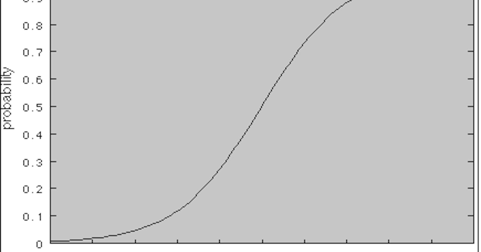
• Use the sigmoid activation function -

• Remember the gradient descent formula for liner regression where Mean squared error was used but we cannot use Mean squared error here so replace with some error E

• Gradient Descent -

• Logistic regression -

• Conditions for E:

• Convex or as convex as possible

• Should be function of theta

• Should be differentiable

• So use, Entropy =

• As we cant use both y hat and y so use cross entropy

• due to second condition add 2 cross entropies CE 1 =

• and CE 2 =

• We get Binary Cross entropy (BCE) =

• So now our formula becomes,

• Using simple chain rule we obtain,

• Now apply Gradient Descent with this formula

So that was about the proof of Logistic regression algorithm now we implement the same above proved algorithm in our code.

Code

We will use the breast cancer data set) to implement our logistic regression algorithm available on the UCI Machine Learning repository.

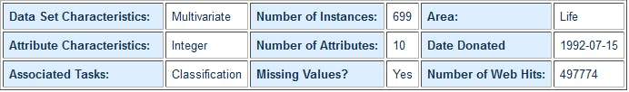data set description

• Import libraries

import numpy as np
import pandas as pd
import random
import seaborn as sns

• Data pre processing Load data, remove empty values. As we are using logistic regression replace 2 and 4 with 0 and 1. Read the data and remove rows with missing values using pandas.

df=pd.read_csv("breast-cancer.data.txt",na_values=['?'])
df.drop(["id"],axis=1,inplace=True)
df["label"].replace(2,0,inplace=True)
df["label"].replace(4,1,inplace=True)
df.dropna(inplace=True)

full_data=df.astype(float).values.tolist()
df.head()

• Visualize data — we will use a pairwise grid for this using seaborn..

sns.pairplot(df)

• Do Principal component analysis for simplified learning.

There is no specific need of doing PCA as we have only 9 features but we get a simpler model eliminating 3 of these features, for code visit the github link.

• Convert data to matrix, concatenate a unit matrix with the complete data matrix. Also make a zero matrix, for the initial theta.

full_data=np.matrix(full_data)
epoch=150000
alpha=0.001
x0=np.ones((full_data.shape[0],1))

data=np.concatenate((x0,full_data),axis=1)
print(data.shape)

theta=np.zeros((1,data.shape[1]-1))
print(theta.shape)
print(theta)

• Create the train-test split

test_size=0.2
X_train=data[:-int(test_size*len(full_data)),:-1]
Y_train=data[:-int(test_size*len(full_data)),-1]
X_test=data[-int(test_size*len(full_data)):,:-1]
Y_test=data[-int(test_size*len(full_data)):,-1]

• Define the code for sigmoid function as mentioned and the BCE.

def sigmoid(Z):
    return 1/(1+np.exp(-Z))

def BCE(X,y,theta):
    pred=sigmoid(np.dot(X,theta.T))
    mcost=-np.array(y)*np.array(np.log(pred))-np.array((1 y))*np.array(np.log(1-pred))

    return mcost.mean()

• Define gradient descent algorithm and also define the number of epochs. Also test the gradient descent by 1 iteration.

def grad_descent(X,y,theta,alpha):
    h=sigmoid(X.dot(theta.T))
    loss=h-y
    dj=(loss.T).dot(X)
    theta -= (alpha/(len(X))*dj)
    return theta

cost=BCE(X_train,Y_train,theta)
print("cost before: ",cost)

theta=grad_descent(X_train,Y_train,theta,alpha)

cost=BCE(X_train,Y_train,theta)
print("cost after: ",cost)

• Define the logistic regression with gradient descent code.

def logistic_reg(epoch,X,y,theta,alpha):
    for ep in range(epoch):
#         update theta 
        theta=grad_descent(X,y,theta,alpha)

#         calculate new loss
        if ((ep+1)%1000 == 0):
            loss=BCE(X,y,theta)
            print("Cost function ",loss)
    return theta

theta=logistic_reg(epoch,X_train,Y_train,theta,alpha)

• Finally test the code,

print(BCE(X_train,Y_train,theta))
print(BCE(X_test,Y_test,theta))

Now we are done with the code

Some other algorithms for same project

1. Multi class Neural Networks

2. Random Forest classifier Project link

GitHub Repo: Here

About me

Rishit Dagli Website LinkedIn