The Ferromagnetic Potts Model

The ferromagnetic Potts model is a canonical example of a Markov random field from statistical physics that is of great probabilistic and algorithmic interest. This is a distribution over all $1$-colorings of the vertices of a graph where monochromatic edges are favored. The algorithmic problem of efficiently sampling approximately from this model is known to be #BIS-hard, and has seen a lot of recent interest. This blog outlinea some recently developed algorithms for approximately sampling from the ferromagnetic Potts model on d-regular weakly expanding graphs. This is achieved by a significantly sharper analysis of standard "polymer methods" using extremal graph theory and applications of Karger's algorithm to count cuts that may be of independent interest. I will give an introduction to all the topics that are relevant to the results. This article is mostly about what I learned from the paper "Algorithms for the ferromagnetic Potts model on expanders" [^carlson2022algorithms]

The Ferromagnetic Potts Model

We start by defining some basic notation:

$G$: finite graph on vertices $V$
$q \in \mathbb{N}$, we are interested in $q$-colourings of the vertices in $G$
$m(\chi)$: number of monochromatic edges induced by a colouring $\chi$
Distribution on colourings given by $p(\chi) \propto exp(\beta \cdot m(\chi))$
$\beta \in \mathbb{R}$: parameter, inverse temperature

Notice that for $\beta < 0$ it means that we take the antiferromagnetic case. Here we talk more about when $\beta > 0$ meaning it is ferromagnetic.

This could have quite some applications:

Modelling: Social networks, physics, chemistry, etc
Markov Random field: Probabilistic Inference
Connection to UGC [^coulson_et_al]
and more.

The Problem

we know $p(\chi) \propto exp(\beta \cdot m(\chi))$

Now for $\beta = 0$ it means that we are doing a uniform $q$-coloring of $V$

For $\beta = -\infty$ we do a uniform proper coloring of $G$

What we need to do is given $G$ and $\beta$, efficiently sample a coloring from this distribution.

$$p(\chi) = \frac{exp(\beta m(\chi))}{\sum_{\chi}exp(\beta m(\chi))}$$

We add the normalizing factor here:

$$\text{Nomalizing factor } = \sum_{\chi}exp(\beta m(\chi))$$

Now we can also say,

$$\sum_{\chi}exp(\beta m(\chi)) =: Z_G(q,\beta)$$

A partition function of the model/distribution is very important for this POV. Our problem is that given $G$ and $\beta$ we want to efficiently sample a color distribution.

We give 2 facts:

It is enough to compute $Z_G(q,\beta)$
#P-hard

We now modify the problem as: Given $G$ and $\beta$, efficiently sample \textbf{approximately} a colouring from this distribution.

$\epsilon$ approximation will have us sample a law from $q$ such that $\mid \mid p-q\mid \mid _{TVD} \leq \epsilon$, thus

$$\mid \mid p-q\mid \mid {TVD} := \frac{1}{2} \sum{\chi} \mid p(\chi) - q(\chi)\mid$$

We modify our original problem template to now be: Given $G$ and $\beta$, efficiently sample $\epsilon$-\textbf{approximately} a colouring from this distribution.

Fully Polynomial Almost Uniform Sampler can allow us to sample $\epsilon$-approximately in $poly(G,\frac{1}{\epsilon})$ time.

Instead Fully Polynomial Time Approximation Scheme: $1 \pm \epsilon$-factor approximation in $poly(G,\frac{1}{\epsilon})$ time.

We can also show for a fact that $FPTAS \iff FPAUS$.

Antiferromagnetic Potts model

The Antiferromagnetic Potts model:

$$p(\chi) \propto exp{\beta \cdot m(\chi)}$$

where $\beta < 0$

Given $G$ and $\beta < 0$, we want to be able to give an FPAUS for this distribution. It is then equivalent to instead work on the problem: given $G$ and $\beta < 0$, give an FPTAS for its partition function $Z_G(q, \beta)$.

From some previous work, we know that there exists a $\beta_c$ such that:

for $\beta < \beta_c$, FPTAS exists
For $\beta < \beta_c$, no FPTAS unless $NP = RP$

We can say that this is #BIS-hard (bipartite independent sets). Thus, doing this is at least as hard as an FPTAS for the number of independent sets in bipartite graphs. If our graph has no bipartiteness then this becomes a NP-hard problem.

For now, let's consider the problem given a bipartite graph $G$, design an FPTAS for the number of individual sets in $G$. This accurately captures the difficulty of: the number of proper $q$-colorings of a bipartite graph for $q \geq 3$, the number of stable matchings, the number of antichains in posets.

Main Results

For our purposes we assume that $G$ is always a $d$-regular graph on $n$ vertices. Now for a set $S \subset V$, we define it's edge boundary as:

$$\triangledown(S) := # (uv \in G \mid u \in S, v \notin S)$$

Now, $G$ is an $\eta$ expander if for every $S \subset V$ of size at most $n/2$, we have $\mid \triangledown(S)\mid \geq \eta\mid S\mid $ . For example we can take a discrete cube $Q_d$ with vertices ${0,1}^d$, $uv$ is an edge if $u$ and $v$ differ in exactly 1 coordinate.

Using a simplification of the Harper's Theorem we can say that $Q_d$ is a $1$-expander [^frankl1981short].

Theorem: For each $\epsilon > 0$ and there is a $d=d(\epsilon)$ and $q = q(\epsilon)$ such that there is an FPTAS for $Z_G(q, \beta)$ where $G$ is a $d$-regular $2$-expander providing the following conditions hold:

$q=poly(d)$
$\beta \notin (2 \pm \epsilon)\frac{ln(q)}{d}$

The main result shown was that

Theorem: For each $\epsilon > 0$, and $d$ large enough, there is an FPTAS for $Z_G(q, \beta)$ where $G$ for the class of $d$-regular triangle-free $1$-expander grpahs providing the following conditions hold:

$q \geq poly(d)$
$\beta \notin (2 \pm \epsilon)\frac{ln(q)}{d}$

This was previously known for:

Stronger expansion and $d = q^{\Omega(d)}$
Higher temperature and $q = d^{\Omega(d)}$

Something to note here is that $q \geq poly(d)$ should not be a necessary condition.

As well as as in the case $\beta \leq (1-\epsilon) \beta_0$ does not require expansion or even that $q \geq poly(d)$.

Potts Distribution

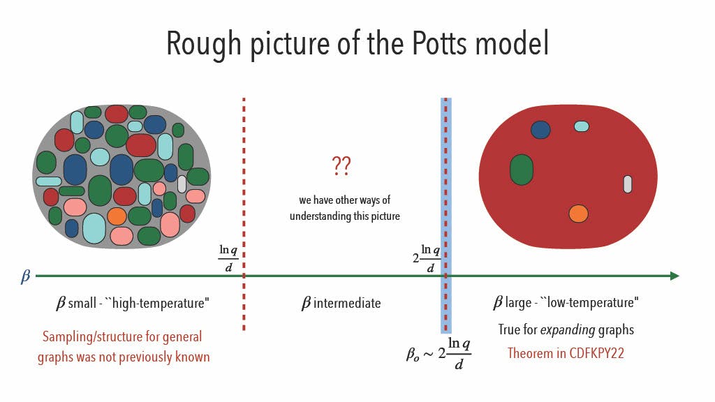
We first write the order-disorder threshold of the ferromagnetic Potts model

$$\beta_0 := ln\left(\frac{q-2}{(q-1)^{1-2/d} - 1}\right)$$

$$\beta_0 = 2 \frac{\ln q}{d} \left(1+O \left( \frac{1}{q} \right)\right)$$

We want to be able to know more about how the Potts distribution looks for $\beta < (1-\epsilon)\beta_0$ and for $\beta > (1+\epsilon)\beta_0$

Results

Another result we have is:

Theorem: For each $\epsilon>0$, let $d$ be large enough $q \geq poly(d)$, and $G$ be a $d$-regular $2$-expander graph on $n$ vertices then,

For $\beta < (1-\epsilon) \beta_0$, every colour class has size $n/q (1 \pm o(1))$ with high probability
For $\beta > (1+\epsilon) \beta_0$, every colour class has size $n-o(n)$ with high probability

The strategy we have, to prove the theorem for $\beta < (1-\epsilon) \beta_0$:

Pass to the Random Cluster Model
Distribution on subsets of edges: $p(A) \propto q^{k(A)} (e^{\beta}-1)^{\mid A\mid }$
$Z_G^{RC}(q, \beta) = Z_G^{Potts}(q, \beta)$
Sampling algorithm: Sample from random cluster model, give each connected component a uniform color
Standard polymer methods + careful enumeration

Polymer Methods

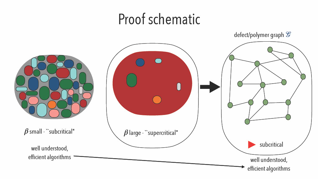
The motivating idea is to visualize the state for $\beta$ large at low temperature as ground state + defects.

Typical Colouring = Ground State + Defects

Polymer methods are pretty useful in such cases. These were first proposed in [^helmuth2019] and originated in statistical physics. We take $G$ to be our defect graph and each node in this represents a defect.

Now using Polymer methods $X \sim _GY$

Ideas is to $ZG(q,\beta) \sim Z{red} + Z{blue}+\dots$ where $Z{red} \approx e^{\beta nd/2}$

$Z{red} e^{-\beta nd/2} = \sum{I \subset V(G)} \prod{\gamma \in I}w{\gamma}$ where $w_{\gamma}$ is the weight of polymer $\gamma$.

We now move towards cluster expansion: multivariate in the $w_{\gamma}$ Taylor expansion of:

$$ln(\sum{I \subset V(G)} \prod{\gamma \in I}w_{\gamma})$$

This is an infinite sum, so convergence is not guaranteed however convergence can be established by verifying the Koteck-Preiss criterion.

We also want to answer how many connected subsets are there of a given edge boundary in an $\eta$-expander?

A heuristic we have is to count the number of such subsets that contain a given vertex $u$: a typical connected subgraph of size $a$ is tree-like, i.e., has edge boundary $a \cdot d$.

Working backward, a typically connected subgraph with edge boundary size $b$ has $O(b/d)$ vertices. The number of such subgraphs $\leq$ number of connected subgraphs of size $O(b/d)$ containing $u$. The original number of subsets is also $\leq$ Number of rooted (at $u$) trees with $O(b/d)$ vertices and maximum degree at most $d = d^{O(b/d)}$. Thus,

Theorem: At most $d^{O(1+1/\eta)b/d}$ connected subsets in an $\eta$ expander that contains $u$ have edge boundary of size at most $b$.

Another question to ask is how many $q$-colorings of an $\eta$-expander induce at most $k$ non-monochromatic edges?

Easiest way is to make $k$ non-monochrimatic edges is to color all but $k/d$ randomly chosen vertices with the same color. Now, $k$ small $\implies$ these vertices likely form an independent set. we now color these $k/d$ vertices arbitrarily. There are:

$${n \choose k/d} q^{k/d+1}$$

ways.

Theorem: For $\eta$-expanders and $q \geq poly(d)$ there are at most $n^4 q^{O(k/d)}$ possible colourings.

Now we also know the maximum value of $ZG(q,\beta)$ over all graphs $G$ with $n$ vertices, $m$ edges, and max degree $d$. This will always be attained when $G$ is a disjoint union of $K{d+1}$ and $K_1$

References

[^carlson2022algorithms]: Carlson, Charlie, et al. "Algorithms for the ferromagnetic Potts model on expanders." 2022 IEEE 63rd Annual Symposium on Foundations of Computer Science (FOCS). IEEE, 2022.

[^coulson_et_al]: Coulson, Matthew, et al. "Statistical physics approaches to Unique Games." arXiv preprint arXiv:1911.01504 (2019).

[^helmuth2019]: Helmuth, Tyler, Will Perkins, and Guus Regts. "Algorithmic pirogov-sinai theory." Proceedings of the 51st Annual ACM SIGACT Symposium on Theory of Computing. 2019.

[^frankl1981short]: Frankl, Peter, and Zoltan Furedi. "A short proof for a theorem of Harper about Hamming-spheres." Discrete Mathematics 34.3 (1981): 311-313.

Rishit Dagli's Blog

Rishit Dagli's Blog

The Ferromagnetic Potts Model

Table of contents